class Airport {
public:
    string code;
    string name;
};Hash Tables
-
A hash table is a data structure that efficiently implements the dictionary abstract data structure with fast
insert,findandremoveoperations.
Dictionary ADT
-
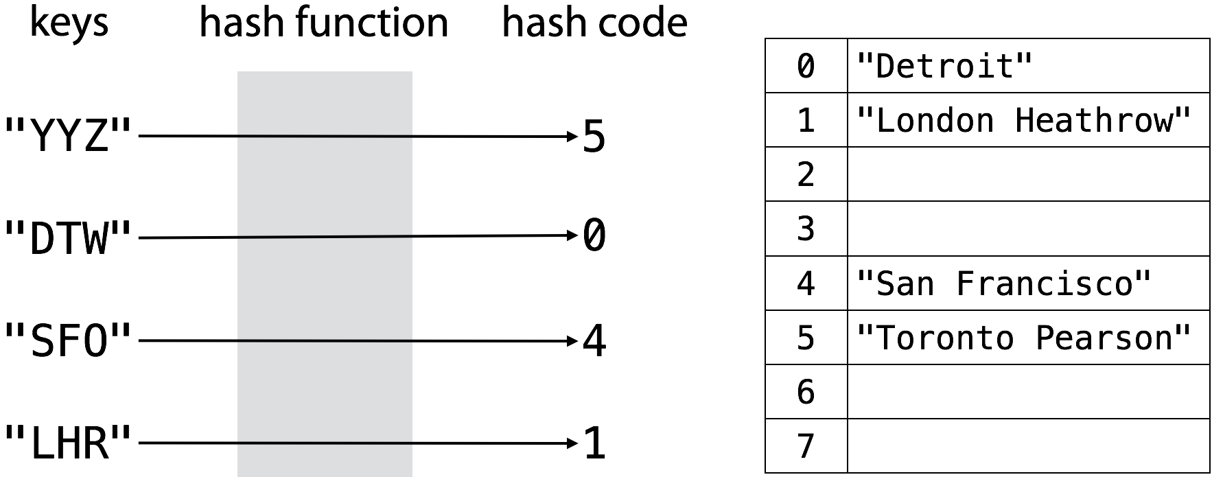
We often want to associate values with keys. For example, we might want to be able to look up an Airport based on its code:
IATA Code Airport DTW
Detroit
LHR
London Heathrow
SFO
San Francisco
YYZ
Toronto Pearson
-
This abstract data structure is called a dictionary and is analogous to an English language dictionary: for each word we want to store a definition. Other names for this ADT are associative array, map, symbol table and key-value pairs.
-
As we maintain a set of key-value pairs, we want to perform three main operations:
-
insert(key, item): insert an item with an associated key.
-
remove(key): remove the item associated with the specified key.
-
find(key): find the item associated with the specified key.
-
-
We could make a simple class or struct to store information about airports.
However, searching for a particular airport by its code in an array of airports would take time if airports are not sorted and time if they are sorted. We want to do better!
-
Hash tables are used when speedy insertion, deletion, and lookup is the priority. In fact, for an ideally tuned hash table, insertion, deletion and lookup can be accomplished in constant time.
Hash Table Structure
-
A hash table is simply an array associated with a function (the hash function). It efficiently implements the dictionary ADT with efficient
insert,removeandfindoperations, each taking expected time. -
The way we are able to achieve this performance is by storing the elements (keys and values) in an array (of size ≥ number of elements). A hash function is used to determine the index where each key-value pair should go in the hash table.
-
Here is the basic pseudocode for the dictionary ADT operations:
insert(key, value):
    index = hashFn(key)
    array[index] = (key, value)

find(key):
    index = hashFn(key)
    return array[index]

remove(key):
    index = hashFn(key)
    array[index] = null
Hash Functions
-
The idea of hashing is to distribute the entries (key/value pairs) across an array.
-
A hash function maps keys to array indices (often called buckets).
where is the universe of keys and is the size of the array.
-
Often, this is a two-step process:
-
We first compute an integer hash code from the key (which can be an object of any type).
-
Then we compress (i.e., reduce) the hash code to a number between and .
-
Hash Codes
-
Let’s consider several ways of generating hash codes for strings.
-
For example, we might want to map airport codes (such as DTW) to airport names like so.
int airportHash(const string &airportCode) {
    if (airportCode.length() != 3) {
        return -1;
    }
    return toupper(airportCode[0]) - 'A';
}
The hash function takes a key (airport code) as input and computes an array index from the intrinsic properties of that key.
Here we return
-1if the airport code is invalid (if it is of a length other than 3). If the airport code is valid, we simply return the alphabetical index of its first letter.Suppose we now wanted to insert Los Angeles Airport (whose code is LAX) into the hash table. LAX hashes to index 11, just as LHR did. This is an example of a collision, the result of multiple keys hashing to the same index.
-
Let’s improve the hash function for airport codes such that each code in the universe of all possible three-letter codes has a unique integer hash code.
int airportHash(const string &airportCode) {
    if (airportCode.length() != 3) {
        return -1;
    }
    return 26 * 26 * (toupper(airportCode[0]) - 'A') +
                26 * (toupper(airportCode[1]) - 'A') +
                     (toupper(airportCode[2]) - 'A');
}
In this function, we ensure that each letter in the airport code has a different effect on the final result by multiplying it by a power of 26. This is a better hash function, but it is prone to collisions, especially if the hash code and the size of the hash table happen to have common factors.
-
In general, a good way to generate hash codes for string
where is a constant . Incidentally, Java uses and 33, 37, 39, and 41 are particularly good choices for a when working with strings that are English words. In fact, in a list of over 50,000 English words taking to be 33, 37, 39, or 41 produces fewer than 7 collisions in each case![1]
This hash code is not as hard to compute for is you might think! Multiplying an integer
xby 31 is equivalent to(x << 5) - x. We can thus write the complete function for computing the hash code for a string:int string hash(const string &s) { int result = 0; for (int i = 0; i < s.length(); i += 1) { result = (result << 5) - result + s[i]; } return result; } -
C++ Standard Library happens to have a functor that computes hash codes:
std::hash<>. Standard specializations exist for all built-in types, and some other standard library types such asstd::stringandstd::thread, and you can provide specializations for your own custom types if you’d like. The unordered associative containers (unordered set, unordered multiset, unordered map and unordered multimap) use specializations of the templatestd::hashas the default hash function.
Compression Functions
-
A hash function’s output (often referred to as just hash), usually a 32-bit integer, is too large for the purpose of a practical application. If used as an array’s index, it would dictate the need for an array of size (~4 billion). And since each array element would at the very least be 4 bytes long (in the case of integers or 32-bit pointers), we would need 4 × 4 billion bytes ≈ 16 GB of memory.
-
And so we need to compress the hash code to reduce it to the size of the array we are using for the hash table.
-
The most common compression function is , where is the compressed hash code that we can use as the index in the array, is the original hash code and is the size of the array (aka the number of “buckets” or “slots”).
-
A problem with this hash function is that patters in keys (e.g., 4, 8, 12, 16) will cause collisions and clusters in the hash table, especially if (number of buckets) is a multiple of of 4. For example, suppose is or . Three quarters of the buckets will never be used.
So should ideally be a prime number if this compression method is used.
-
Here’s a better compressing function:
where and are random integers (chosen once and never changed thereafter) and is a prime number much larger than (the number of buckets in the hash table). In this compression method, multiplying by
a, addingband modding byphelps “mix up” the bits in the number, so that we can then safely mod bym(irrespectively ofm's value) without worrying about creating clusters.
Properties of Hash Functions
-
Since we use the hash function to determine where in the hash table to store a key and where in the hash table to search for the key, it is crucial for a hash function to behave consistently and output the same index for identical inputs.
-
Here are some properties of good hash functions to keep in mind:
-
Uniformly distributes output across the size of the hash table.
-
Generates very different hash codes for inputs that only differ slightly.
-
Employs only very simple, quick operations such as bitwise manipulations.
-
-
Unfortunately, hash codes and compression functions are a somewhat a black art. The ideal hash code and compression function would map each key to a uniformly distributed independently chosen (“random”, in a sense) bucket between and . So the probability of two keys colliding would be .
-
As you saw in the previous examples, it is easy to create hash functions that create more collisions than necessary.
-
Remember that collisions can happen at two steps:
-
At the step of creating the hash code, so that two different keys map to the same hash code. Then, no matter which compression function we use, the hash code will compress to the same slot in the array.
-
The compression method can cause clusters if the keys that we insert have patters and the size of the hash table is not a prime number.
-
Collision Resolution
-
A collision occurs when two keys hash to the same index in the array representing the hash table.
-
Even if your hash table is larger than your dataset and you’ve chosen a good hash function, you need a plan for dealing with collisions if and when they arise. Two common methods of dealing with collisions are probing (open addressing) and separate chaining.
Open Addressing
-
In open addressing (or probing), we store the key-value pairs directly in the array. If a slot is occupied, we find another slot in the array using the hash function.
-
The hash function now takes two arguments: , the key that we are inserting and , the probe number. The hash function thus becomes
where is the universe of keys and is the size of the array.
-
With open addressing, we require that for every key , the probe sequence
be a permutation of , so that every position in the hash table is eventually considered as a slot for a new key as the table fills up.
-
Another constraint on open addressing is that the hash table can no longer hold more elements than there are buckets, so is always true.
-
To insert a new element, we hash its key to get the index of the slot in the array where we should insert, and then check if that slot is available. If it’s empty, we insert the new element, otherwise we call the hash function again to get a new index. We stop when we find an available slot or when we have checked all the slots in the hash table.
The pseudocode for insertion is below:
insert(key, value): i = 0 while i ≠ m: index = hashFn(key, i) if array[index] == null: array[index] = (key, value) return index else: i = i + 1 error "hash table overflow" -
To find an element, we hash its key to get the index of the slot in the array. If the element exists and its key is the same, we insert the value (or the key-value pair), otherwise we call the hash function again to get a new index. We stop when we find a slot that is empty or when we have checked all the slots in the hash table.
The pseudocode for finding an element is below:
find(key, value): i = 0 do: index = hashFn(key, i) if array[index].key == key: return array[index].value else: i = i + 1 while array[index] ≠ null or i ≠ m: error "hash table overflow" -
Removing an element is more difficult. When we delete a key from slot
i, we cannot simply mark it asnull, since that would make thefindoperation stop early and fail to check the elements past this slot. We can solve this problem by marking the slotdeleted(sometimes referred to as “ghost”) instead ofnull:remove(key, value): i = 0 while i ≠ m: index = hashFn(key, i) if array[index].key == key: array[index] = deleted return else: i = i + 1We then modify the
insertoperation to support deleted elements:insert(key, value): i = 0 while i ≠ m: index = hashFn(key, i) if array[index] == null or deleted: array[index] = (key, value) return index else: i = i + 1 error "hash table overflow" -
We will now look at three commonly used techniques to compute the probe sequences required for open addressing: linear probing, quadratic probing, and double hashing.
Linear Probing
-
With linear probing, if a key hashes to the same index as a previously stored key, it is assigned the next available slot in the table.
-
The hash function for linear probing thus becomes
where is the ordinary hash function.
-
So LHR is stored at index 11. Then LAX will be stored at index 12. If we then want to insert MAD (which hashes to 12), it will be stored at index 13.
Let’s insert DTW, SFO, LHR, YYZ, LAX and SYD into a hash table using linear probing as the collision resolution schema. We might end up with a hash table that looks like this:

-
As you can surmise even from this simple example, once a collision occurs, you’ve significantly increased chances that another collision will occur in the same area. This is called clustering, and it’s a serious drawback to linear probing.
-
Worst case insertion, deletion, and lookup times have devolved to , as the next available slot could potentially have been the last slot in the table.
Quadratic Probing
-
Quadratic probing is usually a more efficient algorithm for collision resolution, since it better avoids clustering problem that can occur with linear probing. This is done by increasing the interval between probes using a quadratic polynomial function.
Double Hashing
-
In double hashing, the interval between probes is computed by another hash function.
Separate Chaining
-
In the separate chaining model, the hash table is actually an array of pointers to linked lists. When a collision occurs, the key can be inserted in constant time at the head of the appropriate linked list.
-
If we insert DTW, SFO, LHR, YYZ, LAX and SYD into a hash table and use separate chaining as the collision resolution schema, we’ll this hash table.

-
What happens now when we search for something like LAX in the hash table? We must traverse the entire linked list at index 11. The worst case lookup time for a hash table that uses separate chaining (assuming a uniform hash function) is therefore , where is the size of the hash table.
-
We define load factor , where is the number of items in the hash table and is the size of the array.
-
Since is a constant, is theoretically equivalent to . In the real world, however, is a big improvement over ! A good hash function will maximize this real world improvement.
Dynamic Hashing
-
Sometimes we cannot predict in advance how many elements we will need to store in the hash table. If the load factor gets too large, we are in danger of losing constant-time performance.
-
One solution is to grow the hash table when the load factor becomes too large (typically larger than ). We allocate a new array and move all the elements from the old array into the new one.
-
As we move the elements, keys must be rehashed for the new array of buckets. We cannot just copy the linked lists (if we are using chaining) or re-use the same indices, since the compression function will be different for the new array due to its size.
-
If we use open addressing for collision resolution, then we will clear all the “delete me” (aka “ghost”) elements when we resize the table, as all of the existing elements will get rehashed to the appropriate buckets.
-
In order to keep constant time (although amortized), we grow the hash table by some factor, typically 2. The analysis is very similar to resizing a vector when pushing back.
-
We can also shrink hash tables to free up memory.
If we shrink the hash table by halving its size when load factor becomes , we risk resizing (growing and shrinking) the hash table too often if elements get added and removed, and the number of elements stays around the same. For that reason, it’s best to halve the size of the buckets array when for example.
However in practice, it’s only sometimes worth the effort. You might want to give up a bit of this extra memory to avoid spending time to resize and rehash the elements.
1. Michael T. Goodrich, Roberto Tamassia and Michael H. Goldwasser. 2014. Data Structures and Algorithms in Java. Sixth Edition. Wiley Publishing.